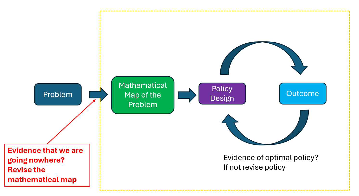
Lately, I’ve been reflecting on how we can prevent “things from getting worse” in a variety of settings — at work, within our families, and even more broadly in society. I’ve come to believe that what truly matters is our ability to course correct: to adjust and improve situations once we understand that they are deteriorating.
The difficulty, of course, lies precisely in that word — understand. Recognizing that things are getting worse is often far from easy. In many cases, it is hard even to articulate clearly what we mean when we say that something is “not going in the right direction.” And in most environments, it can be genuinely difficult to speak up and say, “Something is not right here.”
This is what brings to mind the quote often attributed to Charles Kettering, former head of research at General Motors: “A problem well stated is a problem half solved.” There is considerable wisdom in that statement, particularly when dealing with complex issues and when trying to mobilize groups of people toward meaningful course correction.
Why do I say this? Fundamentally because, in my experience, when problems or opportunities are not well stated, a host of negative dynamics tend to emerge.
- People begin to adapt to problems instead of solving them — a powerful driver of many organizational and social failures.
- A lack of clarity makes it difficult for competent individuals to take the lead.
- Those who have adapted successfully to a flawed situation often resist change, even when the overall impact is negative.
- Morale and energy decline as conditions worsen and collaboration becomes harder.
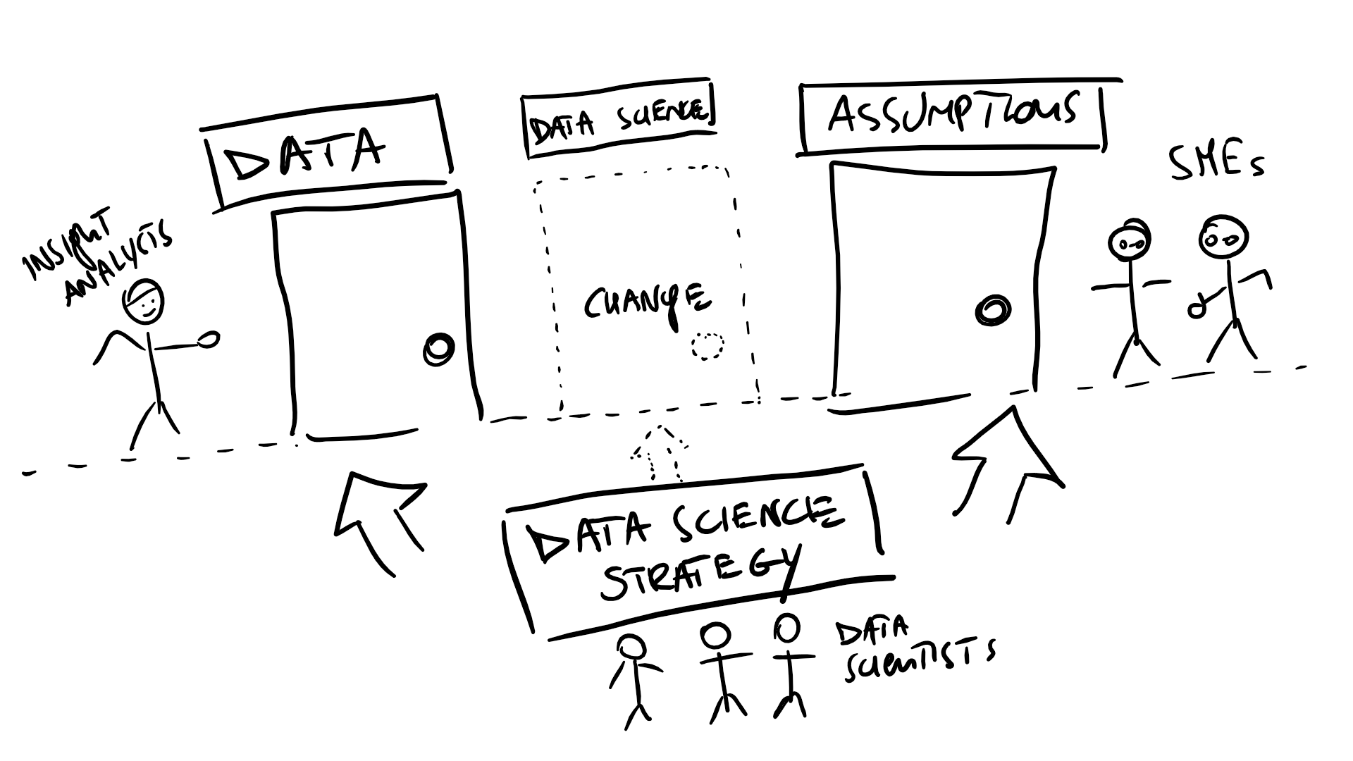
Within the limits of this post, I want to share some thoughts on what can help prevent this outcome. In particular, I want to highlight one family of tools that humans have developed to state problems with exceptional clarity: quantitative models. To be clear, the core point is not about mathematics per se, but about fostering clarity of language and transparency in order to enable course correction. Quantitative models are simply a particularly powerful way to achieve that.
Quantitative models: well-stating problems the hard way
Quantitative models are not always available — after all, they require measurable quantities — but when they are, they are remarkably effective. They force assumptions to be explicit, make key trade-offs visible, and provide a shared and precise language that greatly facilitates collaboration. It is no coincidence that the extraordinary progress of physics, chemistry, and engineering from the 16th century onward coincided with the widespread adoption of mathematical modeling.
In some cases, such as physics, we are even able to state incredibly complex problems with great precision without fully understanding them. Quantum mechanics is a striking example: we can formulate models that answer factual questions with astonishing accuracy, even when their interpretation in plain language remains deeply contested.
Another major benefit of mathematical models is that they uncover relationships that would otherwise remain hidden. A simple example illustrates this.
Suppose you run a sales effort in which you provide services at a loss, hoping that a fraction of prospects will eventually convert to paid customers. You would like to understand how to balance this investment in order to maximize profit. Assume that you are sophisticated enough to have an estimate of the probability of conversion for different prospect profiles.
A natural question arises: up to what probability of conversion should we be willing to provide services at a loss?
At a high level, the answer is intuitive: the gains from converted prospects must offset the losses from those who do not convert. In quantitative terms, this can be written as:

Solving this inequality at breakeven yields the minimum conversion probability required for profitability:

This expression immediately clarifies several things. Profitability depends only on the investment per prospect and the value of a converted customer. And if the investment exceeds the conversion value, there is simply no viable business.
A less obvious insight concerns sensitivity. The conversion threshold depends on investment and conversion value in exactly opposite relative terms: increasing investment by 10% raises the required conversion rate by 10%, while increasing customer value by 10% lowers the threshold by 10%. This kind of elasticity-based reasoning is extremely hard to see without writing the problem down explicitly.
Of course, this model is simplified. In practice, conversion rates often depend on investment — for example, offering a richer free trial may increase the likelihood of conversion. At first glance, this seems to make the problem much harder: the conversion rate depends on investment, but investment decisions depend on the conversion rate.
Yet writing this down actually simplifies the situation. If conversion probability is a function of 

Rather than a fixed threshold, we now have a relationship defining a region of profitability. Far from being an obstacle, this opens the door to optimization: by segmenting prospects by expected value, we can refine investment levels and improve outcomes.
This is a general principle in quantitative modeling: relationships between variables may complicate the mathematics, but they expand the space of possible strategies.
From thresholds to overall profits
So far, the discussion has focused on whether to pursue a given prospect segment. But what about overall profitability once we act?
If conversion rates are not easily influenced by investment, total profits can be written as:

Suppose the baseline conversion rate is 30% and the long-term value of a converted customer is three times the investment. Plugging in the numbers yields a loss: on average, each prospect served generates a loss equal to 10% of the investment.
At this point, several strategic levers are available: improve the product without raising costs, improve it while raising costs but increasing conversion, reduce free-trial costs, or develop targeting models to focus on prospects more likely to convert.
How should a team — say, a group of founders with very different backgrounds — decide which lever to prioritize? Disagreement is inevitable, and mistakes will be made. This is precisely why course correction matters, and why developing a precise language around the problem is so important.
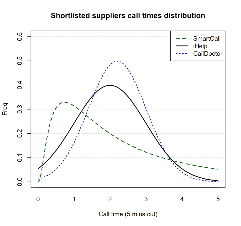
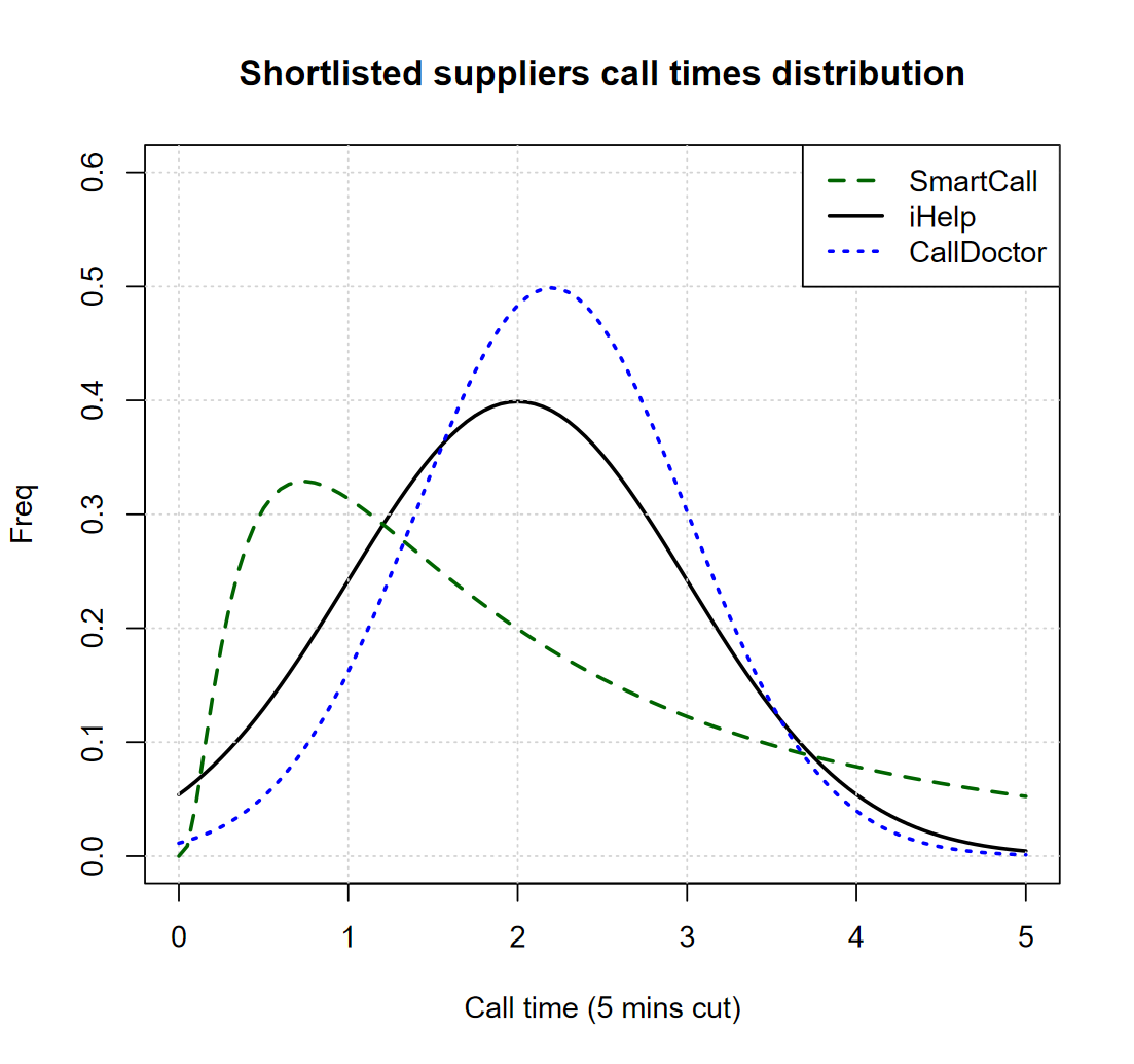
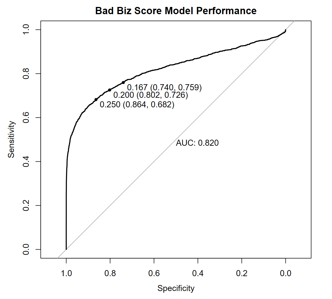
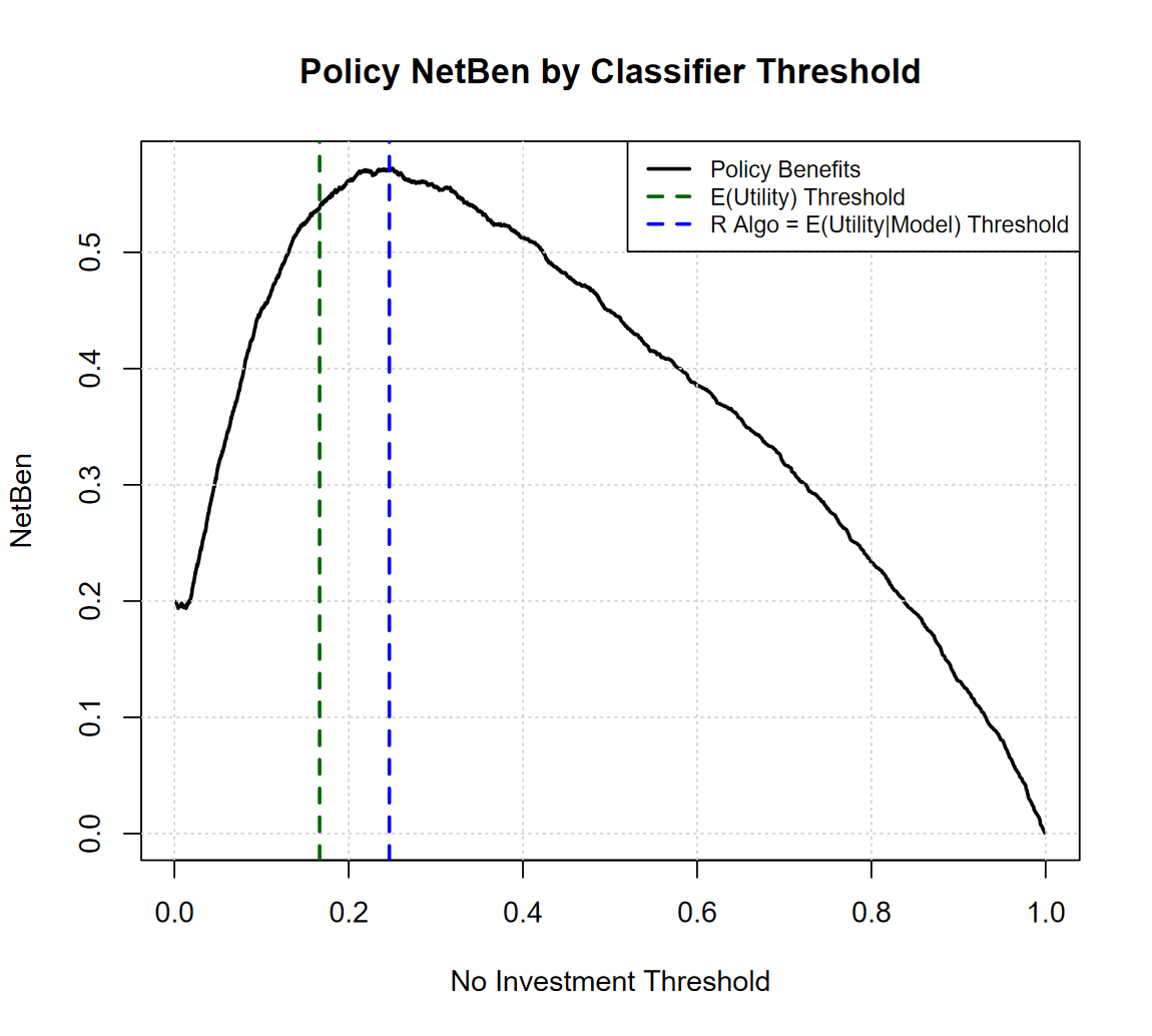
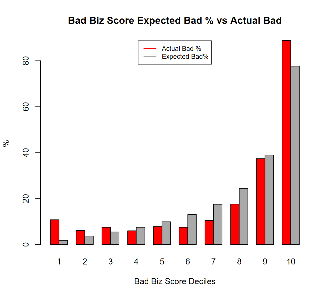
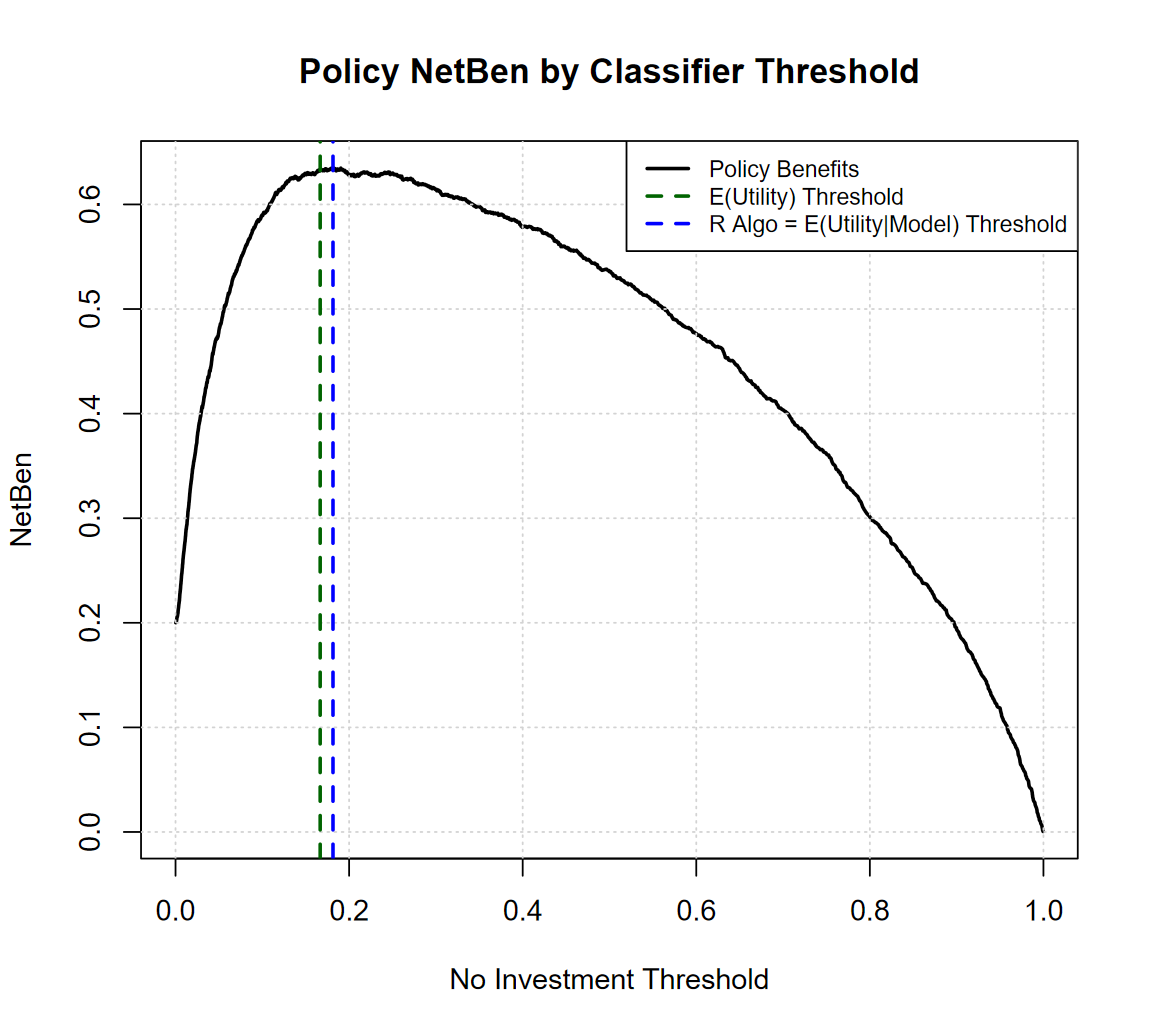
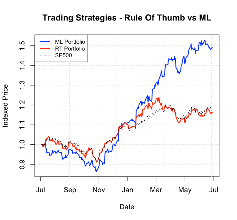
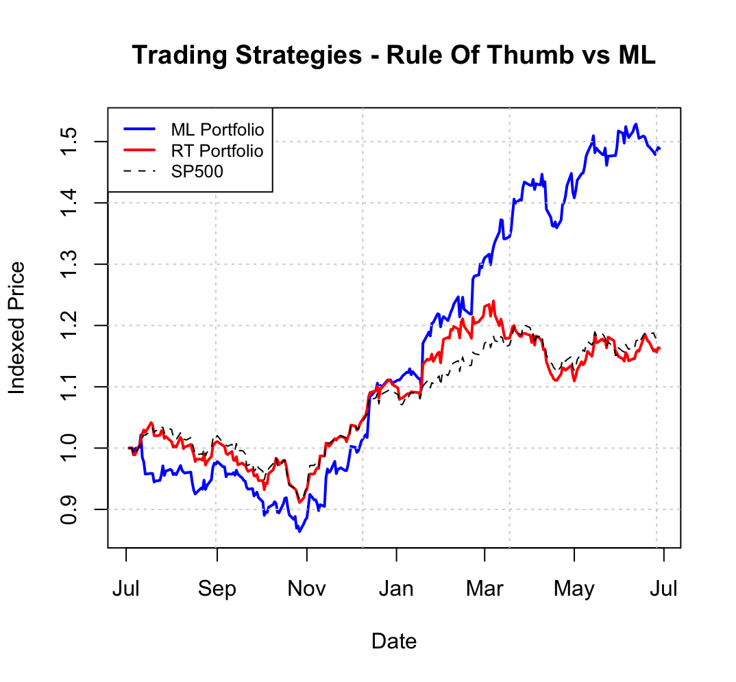
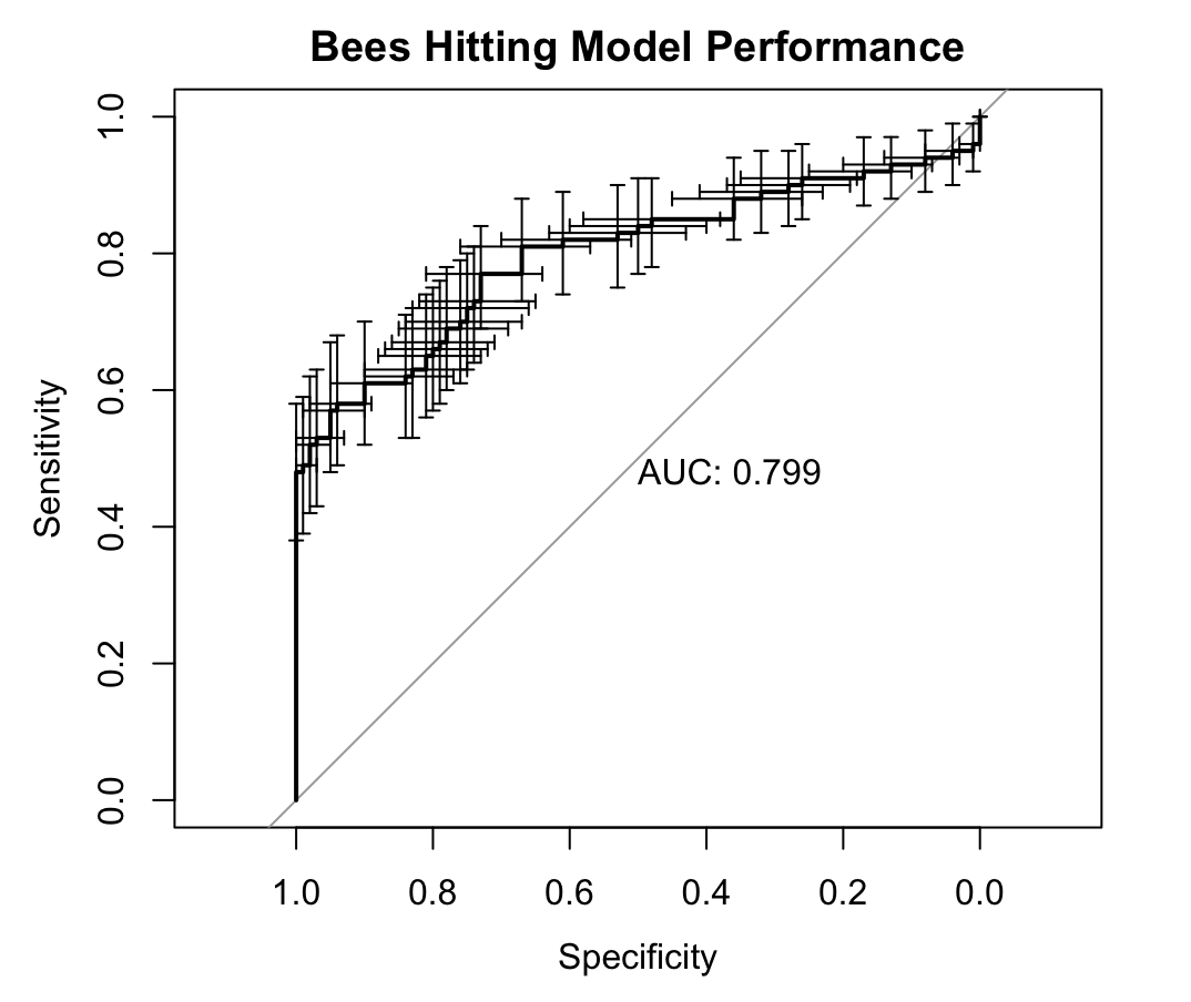
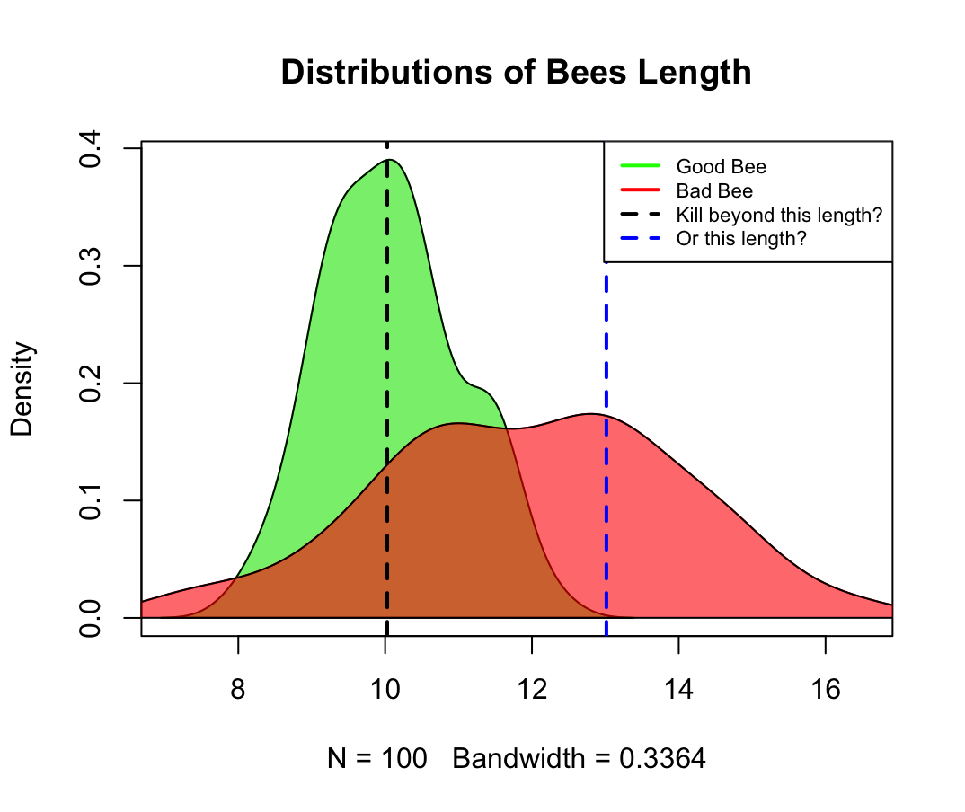
Consider targeting. Suppose we segment the market into two equal-sized groups: Segment A with a 40% conversion rate, and Segment B with a 20% conversion rate. Targeting only Segment A yields positive profits — a substantial improvement driven by a very rough segmentation (equivalent to a two-bin scorecard with a Gini of roughly 23%). See below:

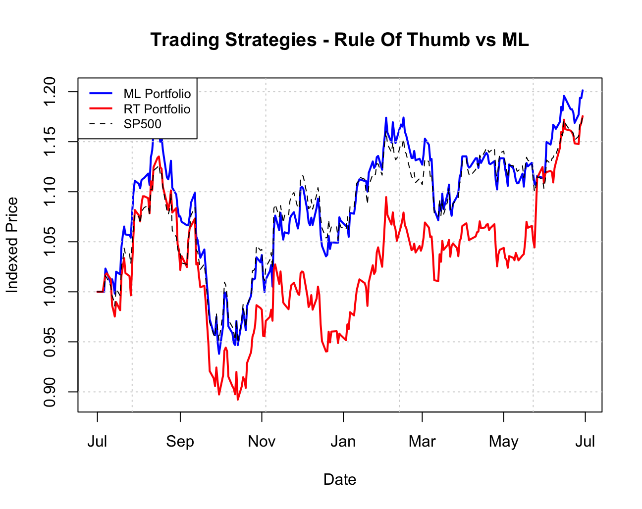
With further work, we could address questions such as: how valuable is improving targeting further? How does that compare with reducing free-trial costs or increasing customer lifetime value? Quantitative models allow us to ask — and answer — these questions systematically.
Clarity, knowledge, and course correction
One might object that quantitative models are difficult for many people to understand, and therefore limit broad participation in decision-making. This is a fair concern. But clarity is never free. Whether expressed mathematically or otherwise, precision requires effort.
Course correction depends on acquiring and applying new knowledge, and conversations about knowledge are rarely easy. We cannot hope to improve conversion through product enhancements without learning what users value most — and learning often requires time, attention, and risk. As Feynman put it, we must “pay attention” at the very least.
Recognizing knowledge, applying it, and revising beliefs accordingly is hard, even for experts. A well-known anecdote from Einstein’s career illustrates this. After developing general relativity, Einstein initially concluded — incorrectly — that gravitational waves did not exist. His paper was rejected due to a mistake, which he initially resisted. Yet within a year, through discussion and correction, he recognized the error and published a revision.
Even giants stumble. Progress depends not on being right the first time, but often on being willing — and able — to correct course.
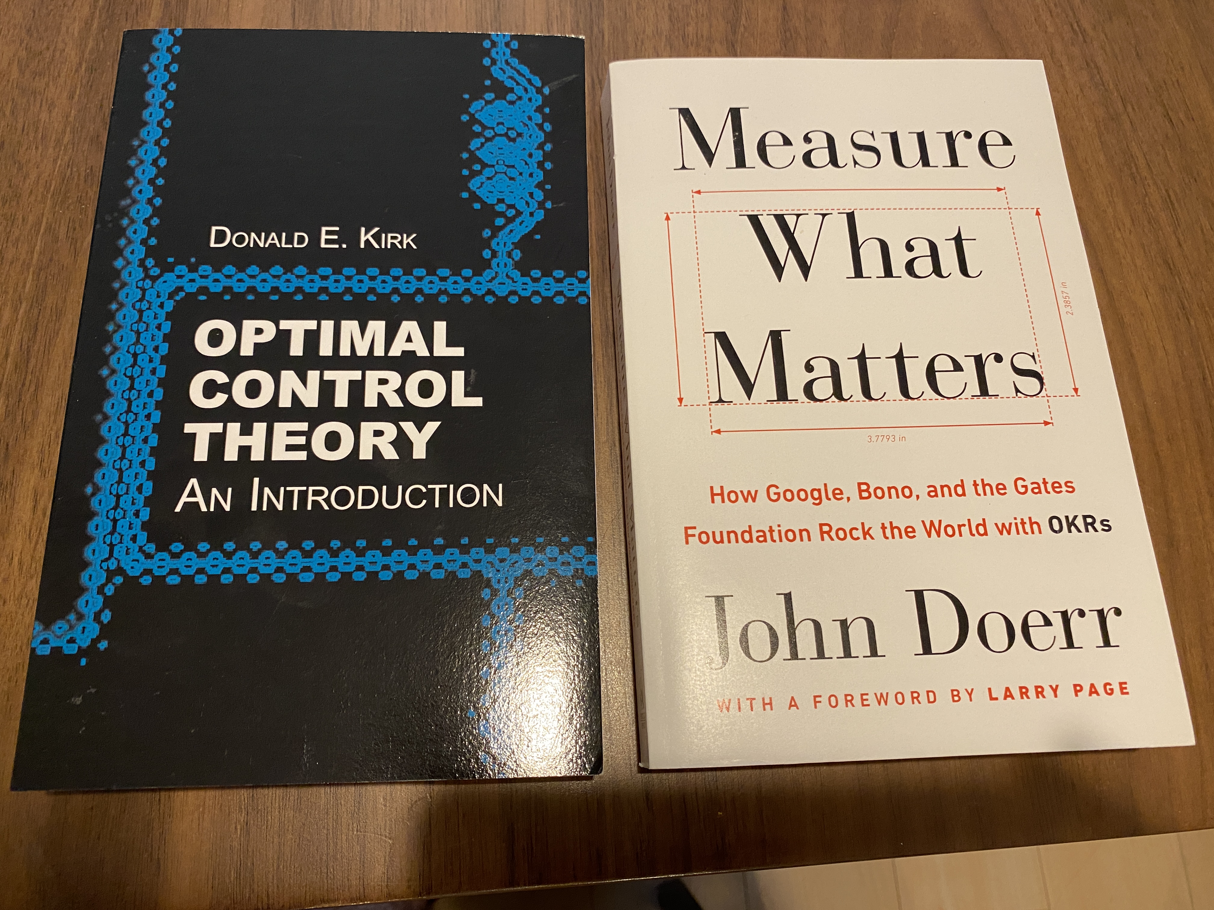
Recommended book on how powerful quantiative models can be:


 :
: