Here I want to discuss about how dealing with uncertainty can be rather unintuitive even in a fairly straightforward example.

Suppose that we are facing questions like below:

Sohuld I make a specific investment where the outcome is uncertain to a certain degree x? How much uncertainty should I be comfortable with?

I want to stress the investment here is generic: buying stock, investing in a marketing campaign, hire personnel, give out a credit card etc.etc. But we are talking of a point in time Yes/No decision (I will cover sequential decisions at a later time).

At first glance this is a pretty easy question to answer, suppose that the expected income when the investment pays out is $1 and the loss is $5 when things go wrong, the equation we generally want to maximize is below ( P(x) being the probability of x):

• E(Income)*P(Pay out)>E(Loss)*P(Loss) which, considering P(Pay out) = 1 – P(Loss), becomes:
• E(Income)*[1-P(Loss)] > E(Loss)*P(Loss) which with some algebra becomes (including a function inversion):
  • P(Loss) < E(Income)/[E(Income) + E(Loss)]

Which is simply a statement that we should go ahead taking risks until the likelihood of gain is greater than the likelihood of a loss. The notation E(variable) means the expectation of the variable, i.e. the most likely outcome.

If we have a situation where the expected income when things go right is $1 and the loss is $5 when things go wrong, it looks like our best action should be to dare until the P(Loss) = 1/(1+5) = 16.6%.

This means that we demand 5 wins every one loss 83.4%/16.6% at least (which should be intuitively right, as the cost of a loss is 5 times that of a win).

Now, I want to point out that this analysis already relies on quite some assumptions:

• 1 – That the expected income is independent of the pay out probability. This is a fair assumption but, in general, the relationship plays a role, e.g., you buy a stock option which is priced low, yet the price is cheap since the pay out probability is considered low by the market. In this case pay out probability and expected income (conditional on pay out) are inversely related. But we also have other situations where the opposite is true (like in credit granting).
• 2 – We have a way to estimate a probability of pay out and loss. This is non trivial, how do we manage that? How would different individuals/models come up with different probabilities?
• 3 – We can make that investment multple times. It does not make sense to guide yourself with probabilities and maximising expected utility, if all you can do is play once. Although this is still the “rational” choice by the book, the topic is debated (see Theory of Decisions Under Uncertainty by Itzhak Gilboa – beautiful book though highly technical)

Ok, assuming the above let us continue with this, and I will show you a condundrum.

Nowadays our problem seems easy, let us get a machine learning model and set the threshold to 16.6%, so that whenever the model tells me that the P(Loss)> 16.6% I won’t go ahead with the investment (or bet, or prospect acquisition). I am glossing over the model details, but it will be a model trained on the useful data for a particular use case (e.g. probability of conversion for a marketing investment, probability of default when giving out credit etc.etc.).

Great, I have created a simulation and I have a classifier performing as below:

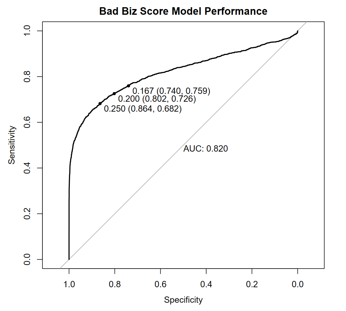
Let me explain the chart briefly:

Sensitivity tells, given a threshold, how good my model is at identifying Bad Biz opportunities, also called the True Positive Rate (where positive means “I am positive this investment is not a good idea”). So, sensitivity should increase as the threshold decreases as we make the model sensitive to fieble signals of Bad Biz. Specificity, on the converse, is how good is the model at being “specific” with its recommendation, meaning how good it is at avoiding collateral damange by giving me, wrongly, a high likelihood of Bad Biz when we are looking at good investments, specificity increases as the threshold increases, as we ask the model to pull the trigger only when the signals are strong.

Overall, in this example, we have a decent model predicting whether the investment I am considering is Bad Biz, i.e. not a good idea, something that will loose money. The Area Under the Curve (AUC) = 0.82 in the chart above (which is called an Receiver Operating Characteristic, or ROC, chart) tells us that the model is 82% likely to correctly rank two investment opportunities in terms of their risk of being a bad business (Bad Biz). This is a global assessment of the model performance across thresholds, and takes into account the sensitivity and specificity we have achieved. The higher the AUC the better the model (on average with respect to the thresholds).

Now, if I ask a common algorithm in R (a statistical programming language) to provide me with the best threshold to guide my strategy, I get below:

> # Best threshold for investment
> coord1 <- min(coords(
+   rocobj,
+   "best",
+   input = "threshold",
+   ret = "threshold",
+   best.weights = c(5, sample_prevalence)
+ ))
> coord1
[1] 0.2466861

So it tells me that I should go as far as 24.6%! That’s pretty different from the “theoretical” threshold we have previously calculated, that one was ~16.6%, what’s going on?

What is going on is that we were not thinking statistically earlier on, but rather probabilistically (mathematically), which is something to consider when it comes to any decision in the real world.

When it comes to actual decisions from models, we need to deal with the model as it is given its actual performance, which is tied to the sample of data we worked with, and how well that data represents “now”. In fact, thinking about it, what happens if your model changes or improves?, or if there are no bad investments out there in a given period? Should we always blindly use the 16.6% probability of Bad Biz? Shouldn’t we react to the actual facts at hand?

The underling issue is that the utility threshold derived theoretically is correct, as mathematics/probability is always correct, nevertheless reality is messy and the score our model gives us is not a probability, but rather a statistical estimate of a probability. In fact the model gives us estimated odds, and odds also need to know the underlying baseline (this is key for the initiated, classifiers scores are not probabilities, but rather they are random variables themselves!).

The clearest way to articulate the actual, empirical outcome, is to use the concept of a policy Net Benefit, which simply measures what value I can expect out of my policy in terms of benefits (from good decisions) and costs (when we get it wrong).

What is the key Net Benefit equation? For a classifier driven policy, depending on threshold x, it is the following:

Net Benefit(x) = TPR(x)*Prevalence*LossPrevented – FPR(x)*(1-Prevalence)*IncomeSuppressed

TPR stands for True Positive Rate, which is simply the number of hits on Bad Biz beyond model threshold x and FPR is, conversely the False Positive Rate, which means that those are investments that are good, but we let go at the threshold x. Prevalence is the general ratio of Bad to Good Biz, regardless of my policy, i.e. if I had no policy that’s what I would get in terms of average bad to good decisions.

So, what will the Net Benefit of my policy be whether we use the expected utility threshold, or the value that the statistical software (R) algorithm gave us? See below:

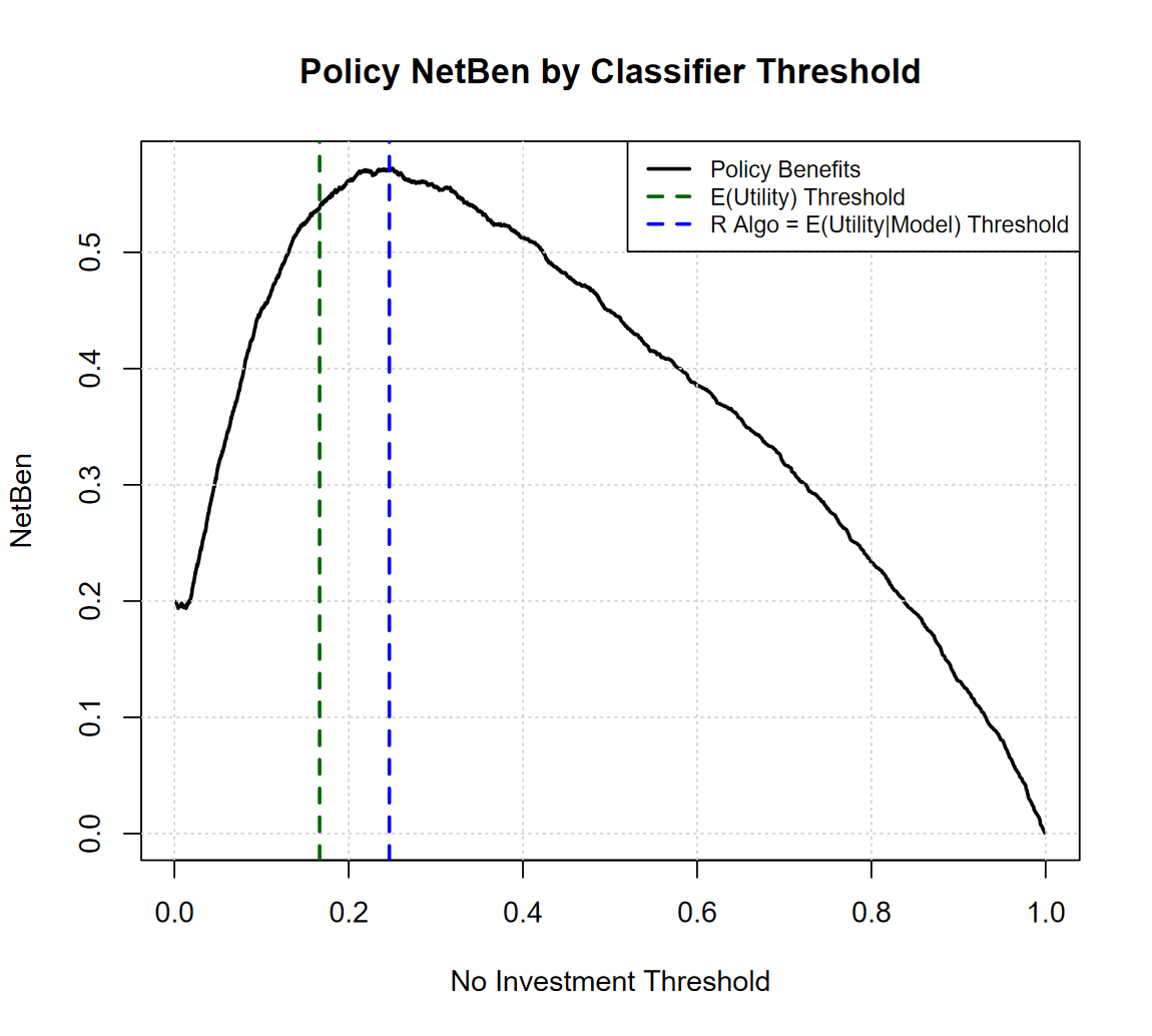
It turns out that R is actually maximizing the Net Benefit equation, which is great, as it is aiming at maximing our expected profits “all” things considered, including the model we are using, and its performance (the optimal threshold can also be derived analytically with some calculus, but won’t go there this time).

The difference in NetBenefit between the two thresholds is high +9% for the “empirical” threshold, this can be a lot of money in a scaled up context.

To recap the overall story is a bit bendy: we have maths, which is correct, and yet, the best action is rather a different one, which is derived statistically. What connects the two thresholds, Maths and Stats derived?

The connection is the classifier itself and “where” the classifier errors are along the utility derived threshold.

On average the classifier scores are perfect, the % of Bad Biz is 20% and the average classifier score for Bad Biz is exacly 20% but… see below:

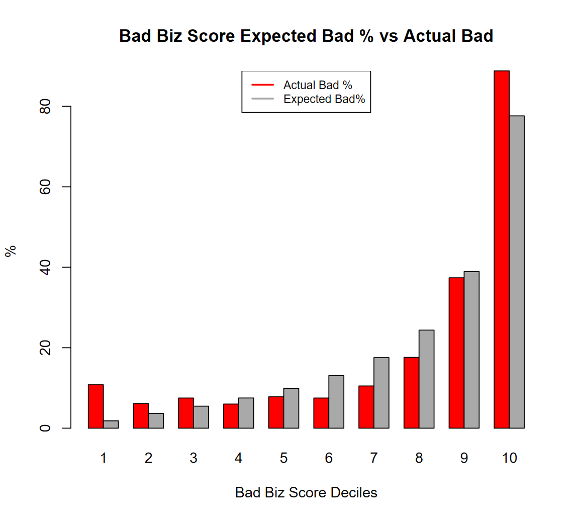
Our “Theoretical” utility threshold happens to be around deciles 6 and 7, where the score (grey bar) overpredicts materally, and this pushes the threshold up. For the threshold determination it does not matter the “global” performance of the model, all that matters is how the model performs around the utility threshold. Nevertheless the issue I have presented above is real, even a well calibrated model will always present distortions, unless it is perfect, and the distortions will be larger when the “Bad” event is rare, therefore we need to deal with it “in practice”.

One thing that I can tell is that if your classifier improves, you can worry less about “Theory vs Reality”, see below how things improve if the classifier achieves 0.87 AUC (from 0.82):

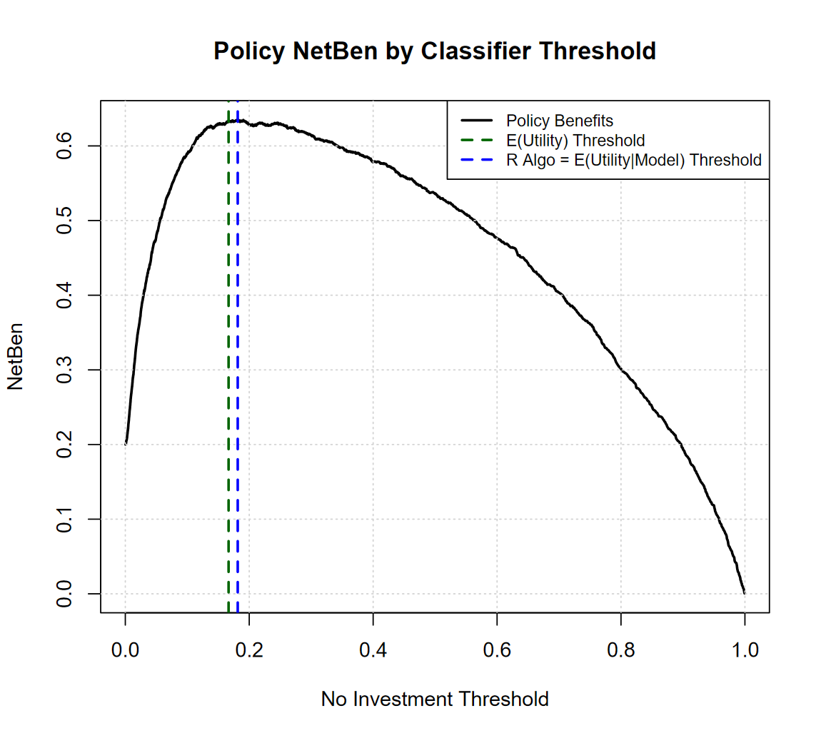
The thresholds get much closer together, and the overall Net Benefit of the policy increases + 16%! (Yes investing in Decision Science is probably worth it).

It is of note that the policy value decreases much steeply to the left (when we are conservative) then to the right (when we take more risk) so -> take more risks when the Bad Biz outcome baseline is low.

It is also worth noticing that, in reality, we do not know that an average loss is going to be $5 and a win $1, nor how noisy things would be around those averages, so, things get much more interesting, and yet the relationship between Maths and Stats needs even more expertise to be dealt with.

Next time, I will try to share more about “sequential” decisions:

What if your choice “now” impacts your future ones? e.g. what if refuting a Biz opportunity from someone will preclude us to do some business with them in the future? Now you might need to rethink your thresholds, as turning down a certain Bad Biz, means turning down several future opportunities.

A key tool to deal with that question is Dynamic Programming (recently rebranded as Reinforcement Learning) a wonderful and powerful idea from the 50s.