Net promoter score is a common measure of customer satisfaction that uses the results of a survey where participants are typically asked how likely they are to recommend a certain brand/company on a 0 to 10 scale (and why they have given the score and what could improve it, but we won’t concentrate on the verbatim).
The score itself is then the percentage of individuals answering 9 or 10 (promoters) minus the percentage of individuals chosing less than 7 (detractors).
There are known ways of correlating NPSs with performance, revenue and profits, therefore it might be the case that, in the context of a research project, a client (internal or external) could ask how they are placed against the competition, but, there is no budget for fieldwork.
Here statistics and analytics might come useful squeezing some information out of existing data.
In particular in this context we use two sources of data:
- Published NPSs by Satmetrix
- Sentiment analysis of tweets sent to the companies under consideration (airlines in this example)
In order to collect the tweets sent to various companies we use a R package called TwitteR developed by Jeff Gentry.
For the ones who don’t know what R, I can breafly say that it is a programming language optimised for statistical tasks (for more information: here)
The scores used for this exercise are from the following 7 airlines:
- Delta nps = 33
- United nps = 10
- JetBlue nps = 56
- SouthwestAir nps = 62
- VirginAmerica nps = 48
- AlaskaAir nps = 47
- AmericanAir nps = 3
Then we use some R code to extract the tweets and calculate the sentiment analysis i.e to see if the tweet sounds like the one a promoter or a detractor would write.
The R package used to measure sentiment is the QDAP by Bryian Goodrich, Dason Kurkiewicz and Tyler Rinker.
Note: In using the Twitter package make sure you have first a twitter account to pretend you are making an app on Twitter to access the API.
I will present the code for scoring the tweets according to two methods:
- Calculating the average polarity (positive, negative) of the overall tweets on an account
- Scoring each tweet individually and then considering a polarity greater than 0.2 as a promoter and less than 0 as a detractor tweet.
Here’s the overall code:
library("stringr")
library("twitteR")
library("qdap")
#go on this website "https://apps.twitter.com/" to get consumer key, secret etc etc logging in with your account..
cred <- (consumer_key ='yourkey',
consumer_secret ='yoursecret',
access_token = 'yourtoken',
access_secret = 'youraccess'
)
# Seems create a function that returns the polarity score of tweets written in English
tweets_polarity <- function(x){
polarity(str_replace_all(unique(sapply(strip_retweets(searchTwitter(x, n=1500, lang = "en", resultType = "recent")), function(x) x$getText())), "[^[:alnum:]]", " "))$group[4]
} # first algorithm: average of tweets polarities
tweets_polarity_2 <- function(x){
y<- c()
y<- unlist(lapply(lapply(lapply(str_replace_all(unique(sapply(strip_retweets(searchTwitter(x, n=700, lang = "en", resultType = "recent")),function(x) x$getText())), "[^[:alnum:]]", " "), polarity), "[[",2),"[[",4))
return(mean(ifelse(y > 0.2, 1, ifelse(y < 0, -1,0))))
} # second algorithm considering polarity > 0.2 as promoters and polarity < 0 as detractors
# Let's also create a list with all the Twitter accounts we want to use the above created function on:
t_accounts<- c("@Delta", "@United", "@JetBlue", "@SouthwestAir", "@VirginAmerica","@AlaskaAir",
"@AmericanAir")
# And use the function on all the accounts on the list
scores<- unlist(sapply(t_accounts, tweets_polarity), use.names = FALSE)# first algorithm
scores_2<- sapply(t_accounts, tweets_polarity_2) # second algorithm
unlist(scores_2)
# Let's also make a vector of NPSs as reported by SATMETRIX
nps<- c(0.33, 0.1, 0.56, 0.62, 0.48, 0.47, 0.03)
# Simple graph first
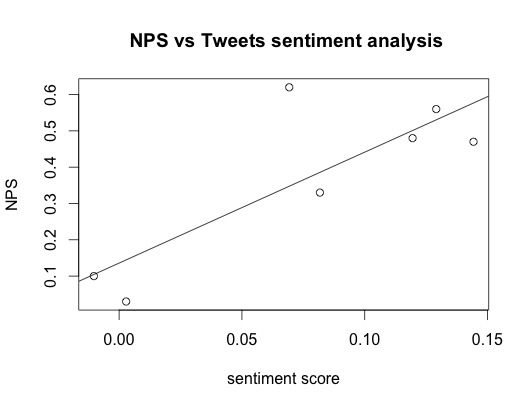
plot(scores, nps, main =" NPS vs Tweets sentiment analysis", xlab = "sentiment score", ylab = "NPS")
abline(model_1)
plot(scores_2, nps, main =" NPS vs Tweets sentiment analysis", xlab = "sentiment score", ylab = "NPS")
# And now the linear models...
model_1.df<- data.frame(nps = nps, scores = scores)
model_2.df<- data.frame(nps = nps, scores = scores_2)
model_1<- lm(nps~scores, method = "qr", data = model_1.df) # with the first algorithm
model_2<- lm(nps~scores, method = "qr", data = model_2.df) # with the second algorithm
#Diagnostics
summary(model_1)
summary(model_2)
plot(model_1)
plot(model_2)
# Prediction of BA and EasyJet nps
ba_ej_score_1<- unlist(sapply(c("@British_Airways", "@easyJet"),tweets_polarity), use.names = FALSE)
predict1<- (model_1, newdata = data.frame(scores = ba_ej_score_1), interval = c("prediction"), level = 0.8)
ba_ej_score_2<- unlist(sapply(c("@British_Airways", "@easyJet"), tweets_polarity_2), use.names = FALSE)
predict_2<- (model_2, newdata = data.frame(scores = ba_ej_score_2 ), interval = c("prediction"), level = 0.8)
So, the code is fairly straightforward. The use of the stringr package is marginal since it is only due to the different encoding of text when using a Mac OS (the code presented works more generally).
But what are the results?
Well, it isn’t the best linear model around as the plot can show:

Nevertheless one could be tricked when calculating the correlation between NPSs and sentiment analysis scores that would return a strong value of 0.81.
Back to the linear model, overall it isn’t that bad and checking the various diagnostic plots we see that the most common rules of thumb in terms of leverages, normality and cook’s distances are not violated.
Now, the model has an adjusted coefficient of explanation that is 0.6 so we don’t expect great predictive power yet the model parameters are significant with a p–value of 0.025.
Conclusions
Back to the task. We have someone at BA asking how they perform against EasyJet and we don’t have budget for any primary research so, we go back to them and say: look, what we can do is to use a cheap and cheerful methodology based on some Twitter sentiment analysis and we are able to say that BA is scoring 0.1 and this gives a 80% confidence interval estimate for their NPS of being between 22 and 67 (the range is from -100 to +100), while EasyJet has a polarity score of 0.01 and this means that their NPS ranges between -7 and 41. Now, as we can see, even at 80% confidence this model is not able to give a clear result saying that BA is better than EasyJet (it does say it is better than American, Delta and United though), but it is only based on 7 data points and, if via some secondary research one can get more NPSs published, it could perform better.
On top of it one could even decide to keep monitoring scores constantly and do some longitudinal modelling too.